Simple Example: Transform and Summarise One Numeric Column
Suppose that we have a column col1 that we wish to
transform in three different ways and compute the five number summary of
the column after the transformations.
library(mverse)
## Loading required package: multiverse
## Loading required package: knitr
##
## Attaching package: 'mverse'
## The following object is masked from 'package:multiverse':
##
##     execute_multiverse
## The following objects are masked from 'package:stats':
##
##     AIC, BIC
library(tibble)
library(dplyr)
##
## Attaching package: 'dplyr'
## The following objects are masked from 'package:stats':
##
##     filter, lag
## The following objects are masked from 'package:base':
##
##     intersect, setdiff, setequal, union
library(ggplot2)
set.seed(6)
df <- tibble(col1 = rnorm(5, 0, 1), col2 = col1 + runif(5))
Step 1: create_multiverse of the data frame
mv <- create_multiverse(df)Step 2: mutate_branch to transform
col1
# Step 2: create a branch - each branch corresponds to a universe

transformation_branch <- mutate_branch(col1 = col1,
                                       col1_t1 = log(abs(col1 + 1)),
                                       col1_t2 = abs(col1))
Step 3: add_mutate_branch to mv
mv <- mv |> add_mutate_branch(transformation_branch)Step 4: execute_multiverse to execute the
transformations
mv <- execute_multiverse(mv)Step 5: Extract Transformed Values from mv
extract to add the column to df_transformed
that labels transformations.
Step 5: use tidyverse to compute the summary and plot
the distribution of each transformation (universe)
df_transformed |>
  group_by(transformation_branch_branch) |>
  summarise(n = n(),
            mean = mean(transformation_branch),
            sd = sd(transformation_branch),
            median = median(transformation_branch),
            IQR = IQR(transformation_branch))
## # A tibble: 3 × 6
##   transformation_branch_branch     n  mean    sd median   IQR
##   <fct>                        <int> <dbl> <dbl>  <dbl> <dbl>
## 1 col1                             5 0.452 0.893  0.270 0.844
## 2 col1_t1                          5 0.179 0.755  0.239 0.601
## 3 col1_t2                          5 0.704 0.658  0.630 0.599

df_transformed |>
  ggplot(aes(x = transformation_branch)) + geom_histogram(bins = 3) +
  facet_wrap(vars(transformation_branch_branch))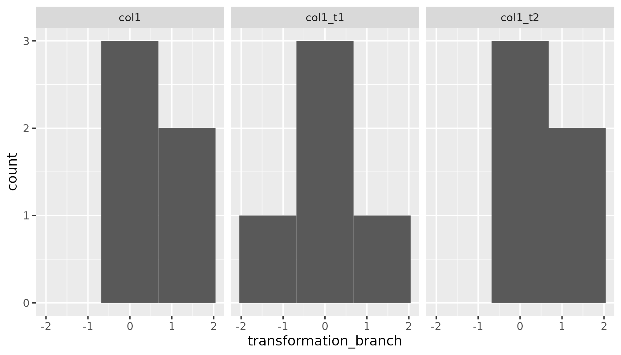
Simple Example: Using mverse to Fit Three Simple Linear
Regression of a Transformed Column
Step 1: create_multiverse of the data frame
mv1 <- create_multiverse(df)Step 2: Create formula_branch of the linear regression
models
formulas <- formula_branch(col2 ~ col1,
                           col2 ~ log(abs(col1 + 1)),
                           col2 ~ abs(col1))
Step 3: add_formula_branch to multiverse of data
frame
mv1 <- mv1 |> add_formula_branch(formulas)Step 3: lm_mverse to compute linear regression models
across the multiverse
lm_mverse(mv1)Step 4: Use summary to extract regression output
summary(mv1)
## # A tibble: 6 × 10
##   universe formulas_branch term    estimate std.error statistic p.value conf.low
##   <fct>    <fct>           <chr>      <dbl>     <dbl>     <dbl>   <dbl>    <dbl>
## 1 1        formulas_1      (Inter…    0.689     0.109      6.31 0.00803   0.342
## 2 1        formulas_1      col1       0.680     0.119      5.71 0.0106    0.301
## 3 2        formulas_2      (Inter…    0.863     0.159      5.43 0.0122    0.358
## 4 2        formulas_2      log(ab…    0.741     0.227      3.26 0.0471    0.0178
## 5 3        formulas_3      (Inter…    0.479     0.330      1.45 0.243    -0.573
## 6 3        formulas_3      abs(co…    0.734     0.360      2.04 0.134    -0.412
## # ℹ 2 more variables: conf.high <dbl>, formulas_branch_code <fct>
Let’s compare using mverse to using
tidyverse and base R to fit the three models.
One way to do this using tidyverse is to create a list
of the model formulas then map the list to lm.
mod1 <- formula(col2 ~ col1)

mod2 <- formula(col2 ~ log(abs(col1 + 1)))

mod3 <- formula(col2 ~ abs(col1))

models <- list(mod1, mod2, mod3)

models |>
  purrr::map(lm, data = df) |>
  purrr::map(broom::tidy) |>
  bind_rows()
## # A tibble: 6 × 5
##   term               estimate std.error statistic p.value
##   <chr>                 <dbl>     <dbl>     <dbl>   <dbl>
## 1 (Intercept)           0.689     0.109      6.31 0.00803
## 2 col1                  0.680     0.119      5.71 0.0106
## 3 (Intercept)           0.863     0.159      5.43 0.0122
## 4 log(abs(col1 + 1))    0.741     0.227      3.26 0.0471
## 5 (Intercept)           0.479     0.330      1.45 0.243
## 6 abs(col1)             0.734     0.360      2.04 0.134
Using base R we can use lappy instead of
modfit <- lapply(models, function(x) lm(x, data = df))

lapply(modfit, function(x) summary(x)[4])
## [[1]]
## [[1]]$coefficients
##              Estimate Std. Error  t value    Pr(>|t|)
## (Intercept) 0.6888352  0.1090963 6.314013 0.008029051
## col1        0.6795288  0.1189216 5.714092 0.010634165
##
##
## [[2]]
## [[2]]$coefficients
##                     Estimate Std. Error  t value   Pr(>|t|)
## (Intercept)        0.8630266  0.1588415 5.433258 0.01223797
## log(abs(col1 + 1)) 0.7409497  0.2272193 3.260945 0.04709792
##
##
## [[3]]
## [[3]]$coefficients
##              Estimate Std. Error  t value  Pr(>|t|)
## (Intercept) 0.4789365  0.3303897 1.449611 0.2430335
## abs(col1)   0.7344512  0.3601450 2.039321 0.1341343
Are Soccer Referees Biased?
In this example, we use a real dataset that demonstrates how
mverse makes it easy to define multiple definitions for a
column and compare the results of the different definitions. We combine
soccer player skin colour ratings by two independent raters
(rater1 and rater2) from soccer
dataset included in mverse.
The data comes from Silberzahn et al. (2014) and contains 146,028 rows of
player-referee pairs. For each player, two independent raters coded
their skin tones on a 5-point scale ranging from very light
skin (0.0) to very dark skin
(1.0). For the purpose of demonstration, we only use a
unique record per player and consider only those with both ratings.
library(mverse)
soccer_bias <- soccer[!is.na(soccer$rater1) & !is.na(soccer$rater2),
                      c("playerShort", "rater1", "rater2")]
soccer_bias <- unique(soccer_bias)
head(soccer_bias)
##          playerShort rater1 rater2
## 1      lucas-wilchez   0.25   0.50
## 2         john-utaka   0.75   0.75
## 6       aaron-hughes   0.25   0.00
## 7 aleksandar-kolarov   0.00   0.25
## 8   alexander-tettey   1.00   1.00
## 9  anders-lindegaard   0.25   0.25
We would like to study the distribution of the player skin tones but the two independent rating do not always match. To combine the two ratings, we may choose to consider the following options:
- the mean numeric value
- the darker rating of the two
- the lighter rating of the two
- the first rating only
- the second rating only
Analysis using Base R and Tidyverse
Let’s first consider how you might study the five options using R
without mverse. First, we define the five options as
separate variables in R.
skin_option_1 <- (soccer_bias$rater1 + soccer_bias$rater2) / 2
skin_option_2 <- ifelse(soccer_bias$rater1 > soccer_bias$rater2,
                        soccer_bias$rater1,
                        soccer_bias$rater2)
skin_option_3 <- ifelse(soccer_bias$rater1 < soccer_bias$rater2,
                        soccer_bias$rater1,
                        soccer_bias$rater2)
skin_option_4 <- soccer_bias$rater1
skin_option_5 <- soccer_bias$rater2
We can plot a histogram to study the distribution of the resulting
skin tone value for each option. Below is the histogram for the first
option (skin_option_1).
library(ggplot2)
ggplot(mapping = aes(x = skin_option_1)) +
  geom_histogram(breaks = seq(0, 1, 0.2),
                 colour = "white") +
  labs(title = "Histogram of player skin tones (Option 1: Mean).",
       x = "Skin Tone", y = "Count")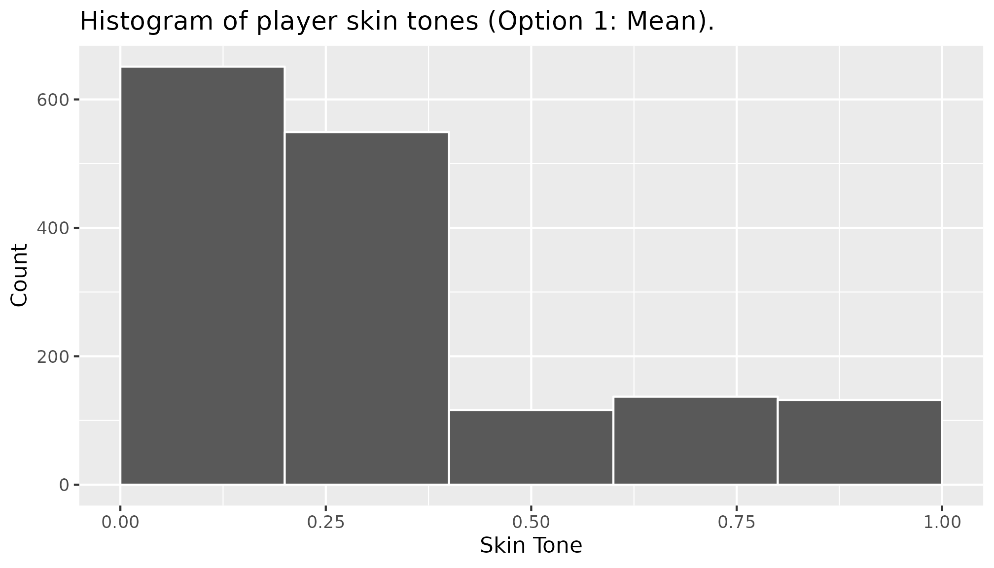
For the remaining four options, we can repeat the step above to examine the distributions, or create a new data frame combining all five options to use in a ggplot as shown below. In both cases, users need to take care of plotting all five manually.
skin_option_all <- data.frame(
  x = c(skin_option_1,
        skin_option_2,
        skin_option_3,
        skin_option_4,
        skin_option_5),
  Option = rep(
    c("Option 1: Mean",
      "Option 2: Max",
      "Option 3: Min",
      "Option 4: Rater 1",
      "Option 5: Rater 2"),
    each = nrow(df)
  )
)
ggplot(data = skin_option_all) +
  geom_histogram(aes(x = x), binwidth = 0.1) +
  labs(title = "Histogram of player skin tones for each option.",
       x = "Skin Tone", y = "Count") +
  facet_wrap(. ~ Option)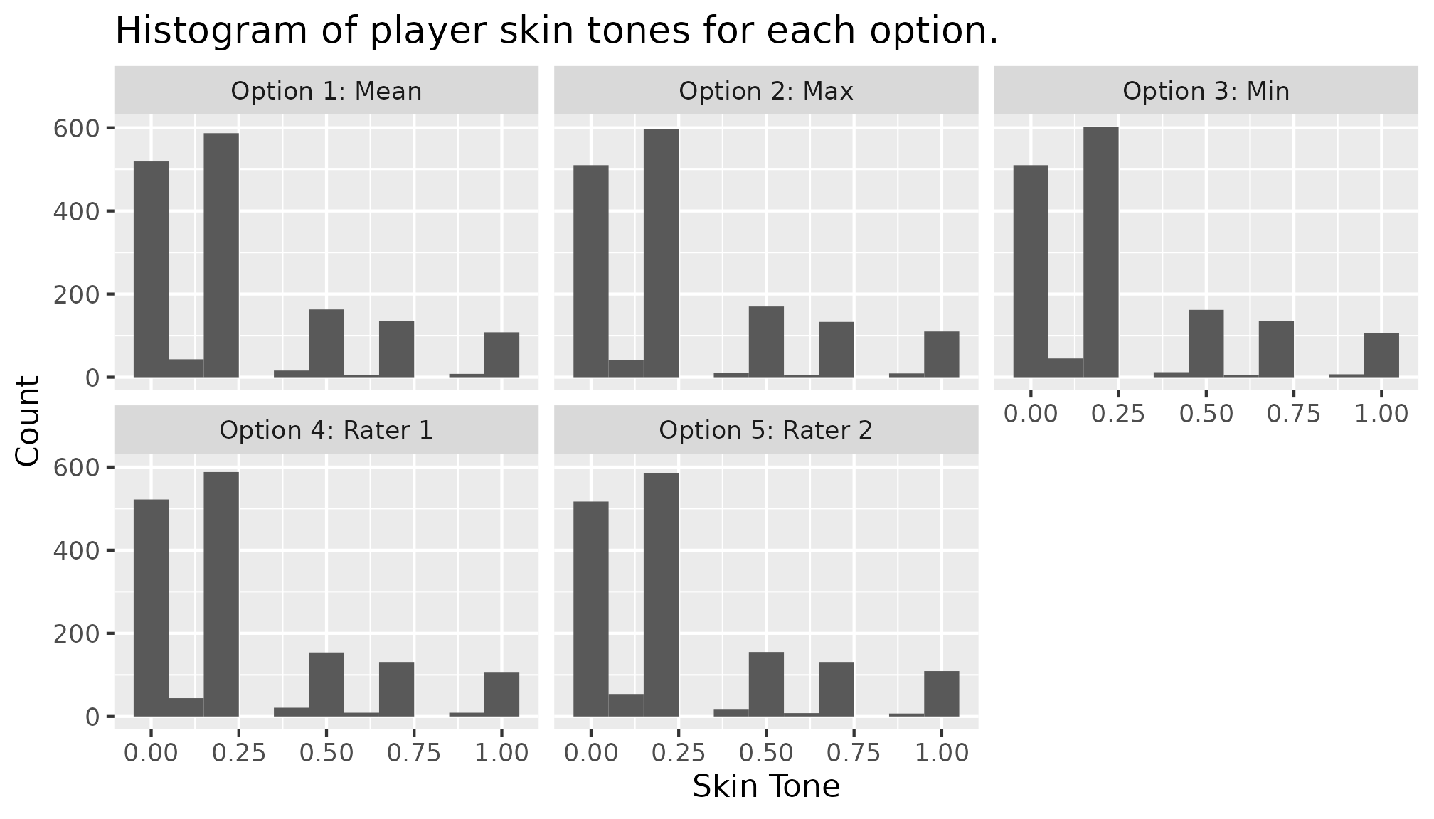
Analysis Using mverse
Branching Using mverse
We now turn to mverse to create the five options above.
First, we define an mverse object with the dataset. Note
that mverse assumes a single dataset for each multiverse
analysis.
soccer_bias_mv <- create_multiverse(soccer_bias)A branch in mverse refers to different
modelling or data wrangling decisions. For example, a mutate branch -
analogous to mutate method in tidyverse’s data
manipulation grammar, lets you define a set of options for defining a
new column in your dataset.
You can create a mutate branch with mutate_branch(). The
syntax for defining the options inside mutate_branch()
follows the tidyverse’s grammar as well.
skin_tone <- mutate_branch(
  (rater1 + rater2) / 2,
  ifelse(rater1 > rater2, rater1, rater2),
  ifelse(rater1 < rater2, rater1, rater2),
  rater1,
  rater2
)
Then add the newly defined mutate branch to the mv
object using add_mutate_branch().
soccer_bias_mv <- soccer_bias_mv |> add_mutate_branch(skin_tone)Adding a branch to a mverse object multiplies the number
of environments defined inside the object so that the environments
capture all unique analysis paths. Without any branches, a
mverse object has a single environment. We call these
environments universes. For example, adding the
skin_tone mutate branch to mv results in
universes inside mv. In each universe, the analysis dataset
now has a new column named skin_tone - the name of the
mutate branch object.
You can check that the mutate branch was added with
summary() method for the mv object. The method
prints a multiverse table that lists all universes with
branches as columns and corresponding options as values defined in the
mv object.
summary(soccer_bias_mv)
## # A tibble: 5 × 3
##   universe skin_tone_branch skin_tone_branch_code
##   <fct>    <fct>            <fct>
## 1 1        skin_tone_1      (rater1 + rater2)/2
## 2 2        skin_tone_2      ifelse(rater1 > rater2, rater1, rater2)
## 3 3        skin_tone_3      ifelse(rater1 < rater2, rater1, rater2)
## 4 4        skin_tone_4      rater1
## 5 5        skin_tone_5      rater2
At this point, the values of the new column skin_tone
are only populated in the first universe. To populate the values for all
universes, we call execute_multiverse.
execute_multiverse(soccer_bias_mv)Summarizing The Distribution Of Each Branch Option
In this section, we now examine and compare the distributions of
skin_tone values between different options. You can extract
the values in each universe using extract(). By default,
the method returns all columns created by a mutate branch across all
universes. In this example, we only have one column -
skin_tone.
branched <- mverse::extract(soccer_bias_mv)branched is a dataset with skin_tone
values. If we want to extract the skin_tone values that
were computed using the average of the two raters then we can filter
branched by skin_tone_branch values equal to
(rater1 + rater2) / 2. Alternatively, we could filter by
universe == 1.
branched |>
  filter(skin_tone_branch == "(rater1 + rater2) / 2") |>
  head()
## [1] universe         skin_tone        skin_tone_branch
## <0 rows> (or 0-length row.names)
The distribution of each method for calculating skin tone can be
computed by grouping the levels of skin_tone_branch.
branched |>
  group_by(skin_tone_branch) |>
  summarise(n = n(),
            mean = mean(skin_tone),
            sd = sd(skin_tone),
            median = median(skin_tone),
            IQR = IQR(skin_tone))
## # A tibble: 5 × 6
##   skin_tone_branch     n  mean    sd median   IQR
##   <fct>            <int> <dbl> <dbl>  <dbl> <dbl>
## 1 skin_tone_1       1585 0.290 0.291   0.25 0.375
## 2 skin_tone_2       1585 0.320 0.297   0.25 0.5
## 3 skin_tone_3       1585 0.259 0.295   0.25 0.25
## 4 skin_tone_4       1585 0.269 0.297   0.25 0.5
## 5 skin_tone_5       1585 0.310 0.297   0.25 0.5
Selecting a random subset of rows data is useful when the multiverse
is large. The frow parameter in extract()
provides the option to extract a random subset of rows in each universe.
It takes a value between 0 and 1 that represent the fraction of values
to extract from each universe. For example, setting
frow = 0.05 returns approximately 5% of values from each
universe (i.e., skin_tone_branch in this case).
frac <- extract(soccer_bias_mv, frow = 0.05)So, each universe is a 20% of the random sample.
frac |>
group_by(universe) |>
tally() |>
mutate(percent = (n / sum(n)) * 100)
## # A tibble: 5 × 3
## universe n percent
## <fct> <int> <dbl>
## 1 1 79 20
## 2 2 79 20
## 3 3 79 20
## 4 4 79 20
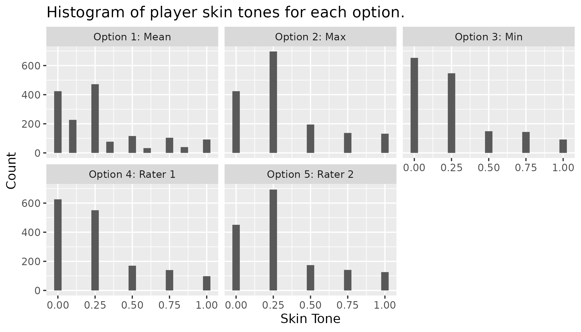
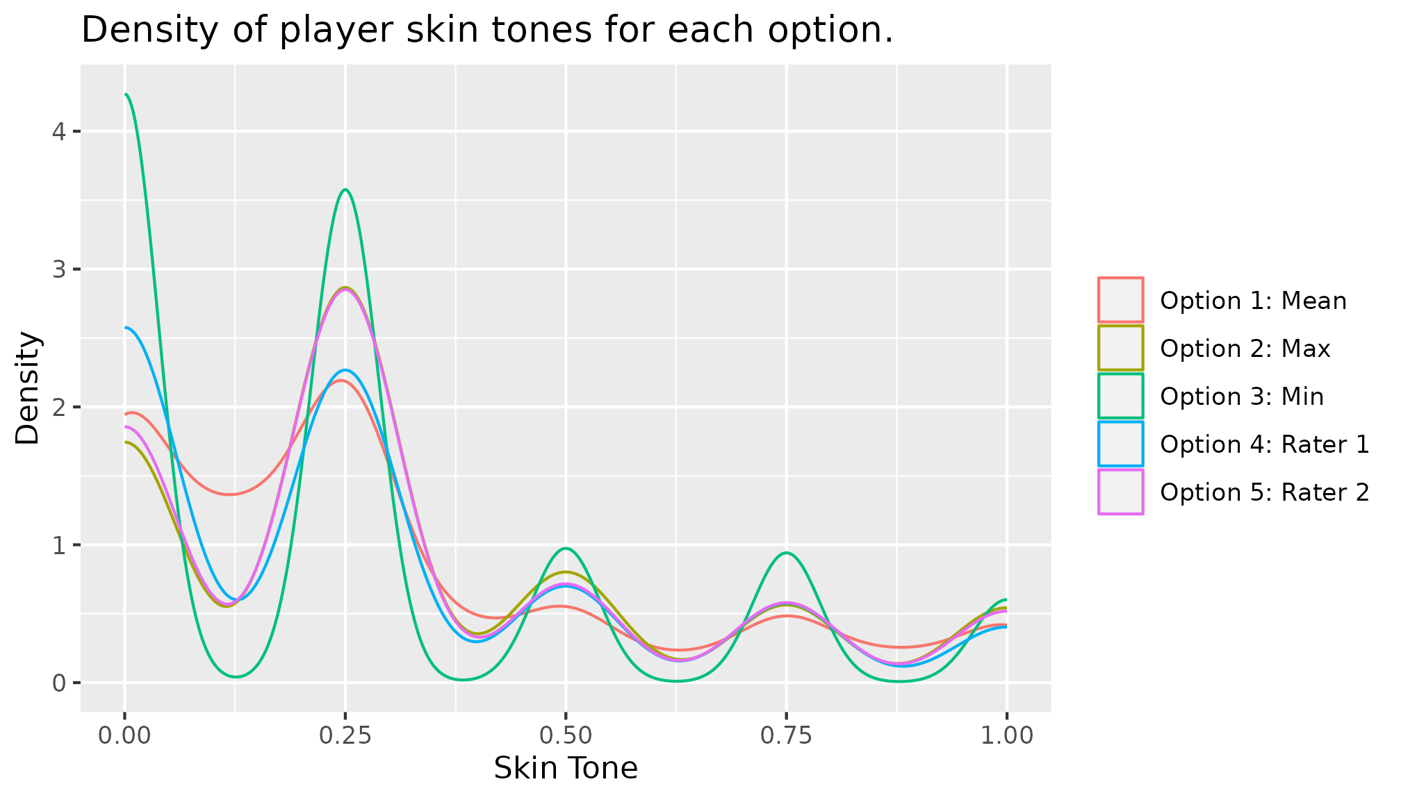
## 5 5 79 20Finally, we can construct plots to compare the distributions of
skin_tone in different universes. For example, you can
overlay density lines on a single plot.
branched |>
  ggplot(mapping = aes(x = skin_tone, color = universe)) +
  geom_density(alpha = 0.2) +
  labs(title = "Density of player skin tones for each option.",
       x = "Skin Tone", y = "Density") +
  scale_color_discrete(
    labels = c("Option 1: Mean",
               "Option 2: Max",
               "Option 3: Min",
               "Option 4: Rater 1",
               "Option 5: Rater 2"),
    name = NULL
  )
Another option is the use ggplot’s
facet_grid function to generate multiple plots in a grid.
facet_wrap(. ~ universe) generates individual plots for
each universe.
branched |>
  ggplot(mapping = aes(x = skin_tone)) +
  geom_histogram(position = "dodge", bins = 21) +
  labs(title = "Histogram of player skin tones for each option.",
       y = "Count", x = "Skin Tone") +
  facet_wrap(
    . ~ universe,
    labeller = labeller(
      universe = c(`1` = "Option 1: Mean",
                   `2` = "Option 2: Max",
                   `3` = "Option 3: Min",
                   `4` = "Option 4: Rater 1",
                   `5` = "Option 5: Rater 2")
    )
  )