GLM Modelling with mverse
Source:vignettes/mverse_intro_glmmodelling.Rmd
mverse_intro_glmmodelling.RmdThis vignette aims to introduce the workflow of a multiverse analysis
with GLM modelling using mverse.
The typical workflow of a multiverse analysis with
mverse is
- Initialize a
multiverseobject with the dataset. - Define all the different data analyses (i.e., analytical decisions) as branches.
- Add defined branches into the
multiverseobject. - Run models, hypothesis tests, and plots.
Exploring The Severity Of Feminine-named Versus Masculine-named Hurricanes
mverse ships with the hurricane dataset
used in Jung et al. (2014).
glimpse(hurricane)
## Rows: 94
## Columns: 14
## $ Year                     <dbl> 1950, 1950, 1952, 1953, 1953, 1954, 1954, 195…
## $ Name                     <chr> "Easy", "King", "Able", "Barbara", "Florence"…
## $ MasFem                   <dbl> 6.777778, 1.388889, 3.833333, 9.833333, 8.333…
## $ MinPressure_before       <dbl> 958, 955, 985, 987, 985, 960, 954, 938, 962, …
## $ Minpressure_Updated_2014 <dbl> 960, 955, 985, 987, 985, 960, 954, 938, 962, …
## $ Gender_MF                <dbl> 1, 0, 0, 1, 1, 1, 1, 1, 1, 1, 0, 1, 1, 1, 1, …
## $ Category                 <dbl> 3, 3, 1, 1, 1, 3, 3, 4, 3, 1, 3, 2, 3, 1, 3, …
## $ alldeaths                <dbl> 2, 4, 3, 1, 0, 60, 20, 20, 0, 200, 7, 15, 1, …
## $ NDAM                     <dbl> 1590, 5350, 150, 58, 15, 19321, 3230, 24260, …
## $ Elapsed.Yrs              <dbl> 63, 63, 61, 60, 60, 59, 59, 59, 58, 58, 58, 5…
## $ Source                   <chr> "MWR", "MWR", "MWR", "MWR", "MWR", "MWR", "MW…
## $ HighestWindSpeed         <dbl> 120, 130, 85, 85, 85, 120, 120, 145, 120, 85,…
## $ MasFem_MTUrk             <dbl> 5.40625, 1.59375, 2.96875, 8.62500, 7.87500, …
## $ NDAM15                   <dbl> 1870, 6030, 170, 65, 18, 21375, 3520, 28500, …
To start a multiverse analysis, first use
create_multiverse to create an mverse object
with hurricane. At this point the multiverse is empty.
hurricane_mv <- create_multiverse(hurricane)Define Branches in the Hurricane Multiverse
Each branch defines a different statistical analysis by using a
subset of data, transforming columns, or a statistical model. Each
combination of these branches defines a “universe”, or analysis path.
Branches are defined using X_branch(...), where
... are expressions that define a data wrangling or
modelling option/analytic decision that you wish to explore, such as
excluding certain hurricane names from an analysis, deriving new
variables for analysis (mutating), or using different models. Once
branches are defined we can look at the impact of the combination of
these decisions.
Branches for Data Manipulation
filter_branch takes logical predicates, and finds the
observations where the condition is TRUE.
The distribution of alldeaths is shown below.
hurricane |>
  ggplot(aes(alldeaths)) +
  geom_histogram(bins = 25) +
  stat_bin(
    aes(label = after_stat(count)), bins = 25,
    geom = "text", vjust = -.7, size = 2
  )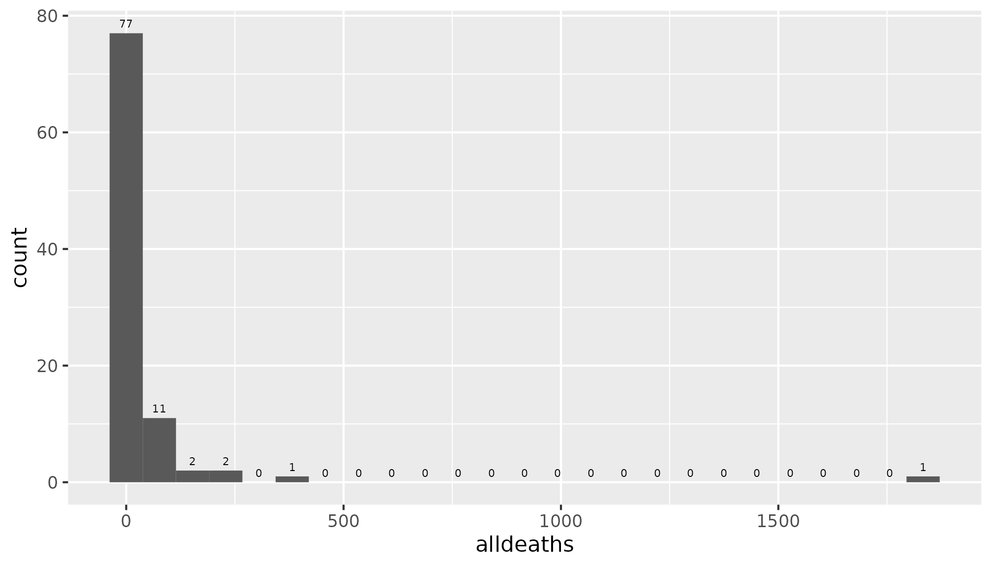
It looks like there are a few outliers. Let’s find out the names of these hurricanes.
hurricane |>
  filter(alldeaths > median(alldeaths)) |>
  arrange(desc(alldeaths)) |>
  select(Name, alldeaths) |>
  head()
## # A tibble: 6 × 2
##   Name    alldeaths
##   <chr>       <dbl>
## 1 Katrina      1833
## 2 Audrey        416
## 3 Camille       256
## 4 Diane         200
## 5 Sandy         159
## 6 Agnes         117
filter_branch() can be used to exclude outliers.
Excluding hurricane Katrina or Audrey removes
the hurricanes with the most deaths.
death_outliers <- filter_branch(
  none = TRUE,
  Katrina = Name != "Katrina",
  KatrinaAudrey = !(Name %in% c("Katrina", "Audrey"))
)
Now, let’s add this branch to hurricane_mv.
hurricane_mv <- hurricane_mv |> add_filter_branch(death_outliers)

summary(hurricane_mv)
## # A tibble: 3 × 3
##   universe death_outliers_branch death_outliers_branch_code
##   <fct>    <fct>                 <fct>
## 1 1        none                  "TRUE"
## 2 2        Katrina               "Name != \"Katrina\""
## 3 3        KatrinaAudrey         "!(Name %in% c(\"Katrina\", \"Audrey\"))"
mutate_branch() takes expressions that can modify data
columns, and can be used to provide different definitions or
transformations of a column.
Consider two different definitions of femininity:
Gender_MF is a binary classification of gender, and
MasFem is a continuous rating of Femininity.
femininity <- mutate_branch(binary = Gender_MF,
                            continuous = MasFem)
Consider normalized damage (NDAM) and the log of
NDAM.
damage <- mutate_branch(original = NDAM,
                        log = log(NDAM))
Now, let’s add these branches to hurricane_mv.
hurricane_mv <- hurricane_mv |> add_mutate_branch(femininity, damage)

summary(hurricane_mv)
## # A tibble: 12 × 7
##    universe death_outliers_branch femininity_branch damage_branch
##    <fct>    <fct>                 <fct>             <fct>
##  1 1        none                  binary            original
##  2 2        none                  binary            log
##  3 3        none                  continuous        original
##  4 4        none                  continuous        log
##  5 5        Katrina               binary            original
##  6 6        Katrina               binary            log
##  7 7        Katrina               continuous        original
##  8 8        Katrina               continuous        log
##  9 9        KatrinaAudrey         binary            original
## 10 10       KatrinaAudrey         binary            log
## 11 11       KatrinaAudrey         continuous        original
## 12 12       KatrinaAudrey         continuous        log
## # ℹ 3 more variables: death_outliers_branch_code <fct>,
## #   femininity_branch_code <fct>, damage_branch_code <fct>
Each row of the multiverse hurricane_mv corresponds to
each combination of death_outliers (3),
femininity (2), and damage (2) for a total of
combinations.
GLM Branches for Modelling
mverse can define different glm() models as
branches. The formula for a glm model (e.g.,
y ~ x) can be defined using formula_branch,
and family_branch defines the member of the exponential
family used via a family object.
We can create formulas using the branches above or simply use the
columns in dataframe. If we use the branches depvars,
damage, and depvars in a formula such as
depvars ~ damage + femininity
We can add it to hurricane_mv with
add_formula_branch().
models <- formula_branch(alldeaths ~ damage + femininity)

hurricane_mv <- hurricane_mv |> add_formula_branch(models)

summary(hurricane_mv)
## # A tibble: 12 × 9
##    universe death_outliers_branch femininity_branch damage_branch models_branch
##    <fct>    <fct>                 <fct>             <fct>         <fct>
##  1 1        none                  binary            original      models_1
##  2 2        none                  binary            log           models_1
##  3 3        none                  continuous        original      models_1
##  4 4        none                  continuous        log           models_1
##  5 5        Katrina               binary            original      models_1
##  6 6        Katrina               binary            log           models_1
##  7 7        Katrina               continuous        original      models_1
##  8 8        Katrina               continuous        log           models_1
##  9 9        KatrinaAudrey         binary            original      models_1
## 10 10       KatrinaAudrey         binary            log           models_1
## 11 11       KatrinaAudrey         continuous        original      models_1
## 12 12       KatrinaAudrey         continuous        log           models_1
## # ℹ 4 more variables: death_outliers_branch_code <fct>,
## #   femininity_branch_code <fct>, damage_branch_code <fct>,
## #   models_branch_code <fct>
Finally, let’s create a family_branch() that defines two
different members of the Exponential family as branches.
distributions <- family_branch(poisson, gaussian)Adding this branch to hurricane_mv with
add_family_branch().
hurricane_mv <- hurricane_mv |> add_family_branch(distributions)

summary(hurricane_mv)
## # A tibble: 24 × 11
##    universe death_outliers_branch femininity_branch damage_branch models_branch
##    <fct>    <fct>                 <fct>             <fct>         <fct>
##  1 1        none                  binary            original      models_1
##  2 2        none                  binary            original      models_1
##  3 3        none                  binary            log           models_1
##  4 4        none                  binary            log           models_1
##  5 5        none                  continuous        original      models_1
##  6 6        none                  continuous        original      models_1
##  7 7        none                  continuous        log           models_1
##  8 8        none                  continuous        log           models_1
##  9 9        Katrina               binary            original      models_1
## 10 10       Katrina               binary            original      models_1
## # ℹ 14 more rows
## # ℹ 6 more variables: distributions_branch <fct>,
## #   death_outliers_branch_code <fct>, femininity_branch_code <fct>,
## #   damage_branch_code <fct>, models_branch_code <fct>,
## #   distributions_branch_code <fct>
Now, we have different combinations.
multiverse_tree can be used to view
hurricane_mv. The tree below shows that
alldeaths is modelled using both Gaussian and Poisson
distributions.
multiverse_tree(hurricane_mv, label = "code", label_size = 4,
                branches = c("models", "distributions"))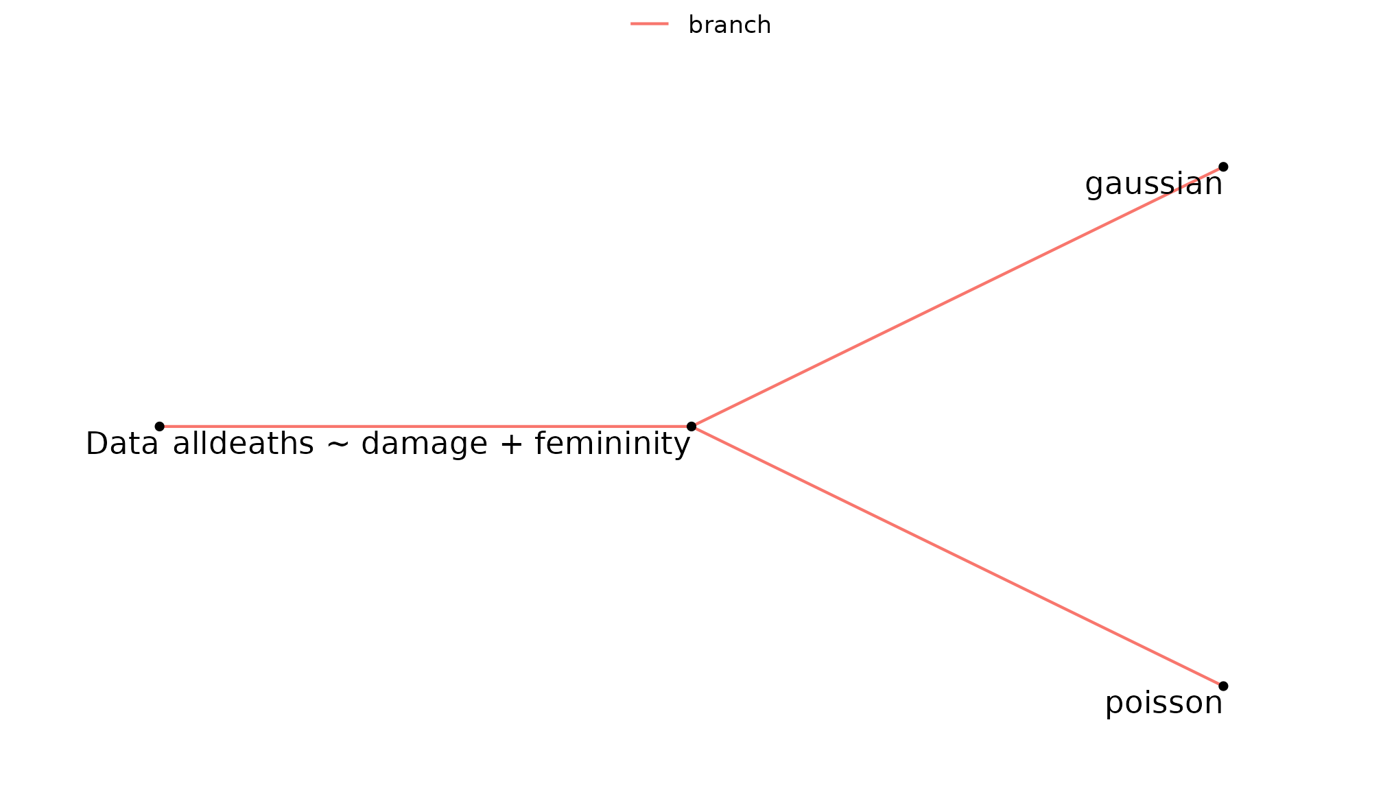
glm_mverse(hurricane_mv)

glm_summary <- summary(hurricane_mv)

glm_summary
## # A tibble: 72 × 18
##    universe death_outliers_branch femininity_branch damage_branch models_branch
##    <fct>    <fct>                 <fct>             <fct>         <fct>
##  1 1        none                  binary            original      models_1
##  2 1        none                  binary            original      models_1
##  3 1        none                  binary            original      models_1
##  4 2        none                  binary            original      models_1
##  5 2        none                  binary            original      models_1
##  6 2        none                  binary            original      models_1
##  7 3        none                  binary            log           models_1
##  8 3        none                  binary            log           models_1
##  9 3        none                  binary            log           models_1
## 10 4        none                  binary            log           models_1
## # ℹ 62 more rows
## # ℹ 13 more variables: distributions_branch <fct>, term <chr>, estimate <dbl>,
## #   std.error <dbl>, statistic <dbl>, p.value <dbl>, conf.low <dbl>,
## #   conf.high <dbl>, death_outliers_branch_code <fct>,
## #   femininity_branch_code <fct>, damage_branch_code <fct>,
## #   models_branch_code <fct>, distributions_branch_code <fct>
Each model has three rows, each corresponding to a summary of a model coefficient.
The specification curve for the coefficient of
femininity is shown below.
spec_summary(hurricane_mv, var = "femininity") |>
  spec_curve(label = "code", spec_matrix_spacing = 4) +
  labs(colour = "Significant at 0.05") +
  theme(legend.position = "top")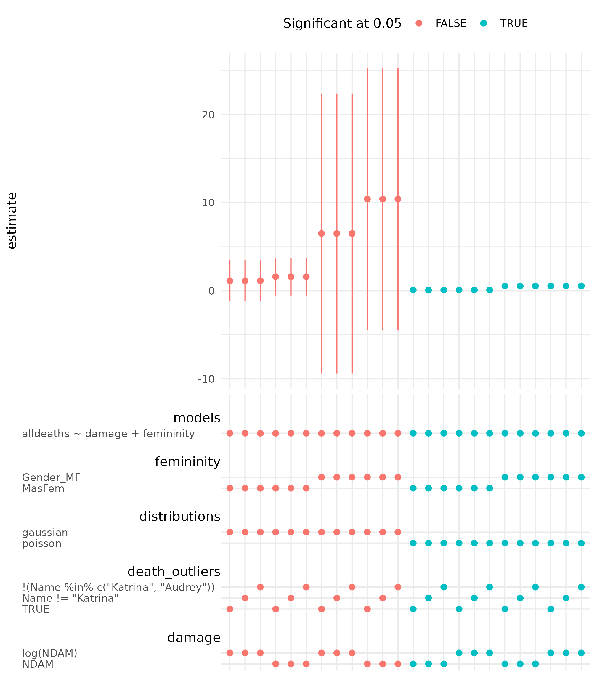
Condition Branches
The assumption that alldeaths follows a Normal
distribution is tenuous, but transforming the alldeaths
using
could result in a dependent variable that is closer to a Normal
distribution.
hurricane |>
  ggplot(aes(sample = alldeaths)) +
  stat_qq() +
  stat_qq_line()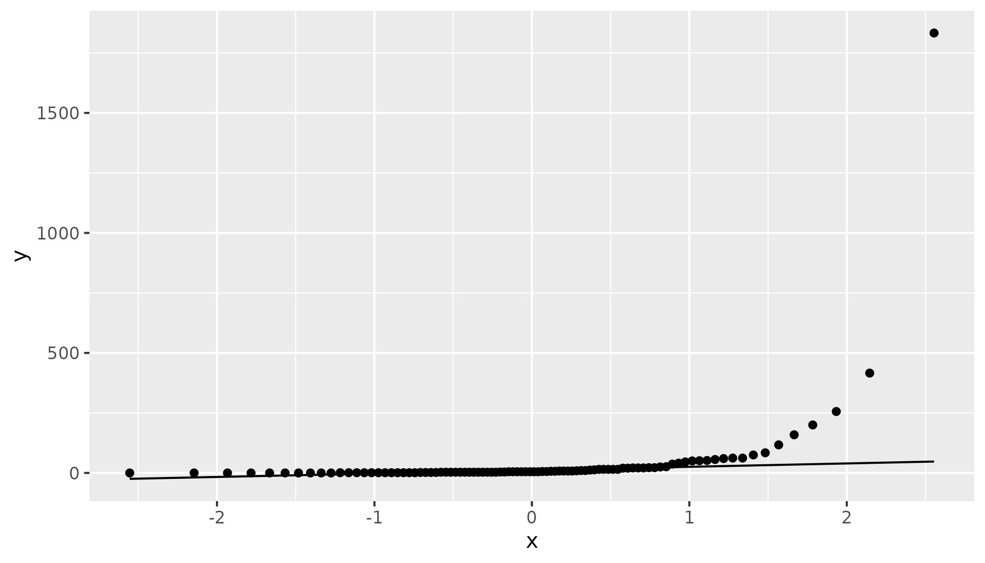
hurricane |>
  mutate(logd = log(alldeaths + 1)) |>
  ggplot(aes(sample = logd)) +
  stat_qq() +
  stat_qq_line()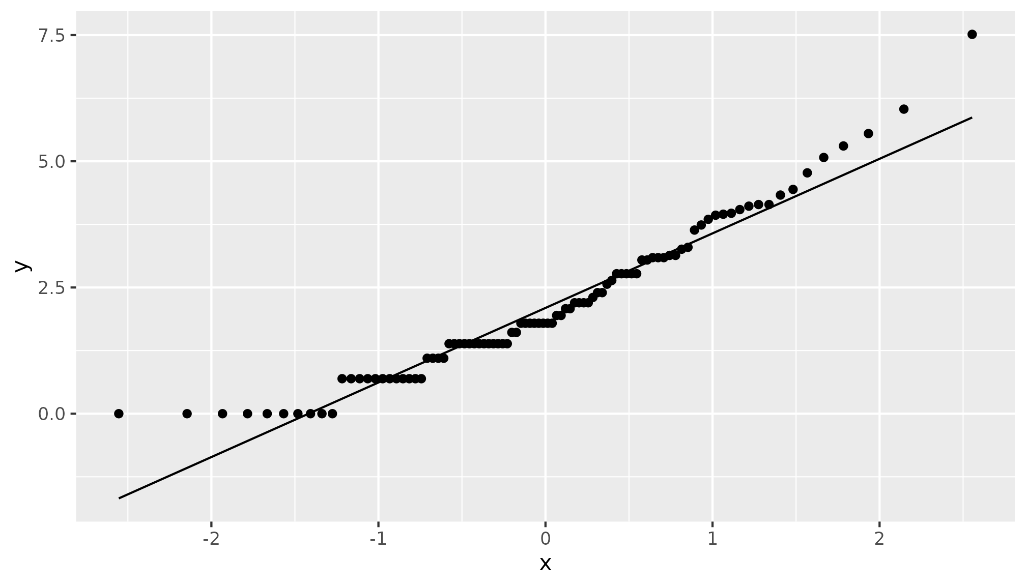
Let’s set up a similar multiverse analysis to the one above.
hurricane_mv <- create_multiverse(hurricane)

dep_var <- mutate_branch(alldeaths, log(alldeaths + 1))

femininity <- mutate_branch(binary_gender = Gender_MF,
                            cts_gender = MasFem)

damage <- mutate_branch(damage_orig = NDAM,
                        damage_log = log(NDAM))

models <- formula_branch(dep_var ~ damage + femininity)

distributions <- family_branch(poisson, gaussian)

hurricane_mv <- hurricane_mv |>
  add_mutate_branch(dep_var, femininity, damage) |>
  add_formula_branch(models) |>
  add_family_branch(distributions)
Using multiverse_tree() to display the multiverse tree
of dep_var and distributions shows that
log(alldeaths + 1) and alldeaths will be
modelled as both Gaussian and Poisson.
multiverse_tree(hurricane_mv, label = "code", c("dep_var", "distributions"))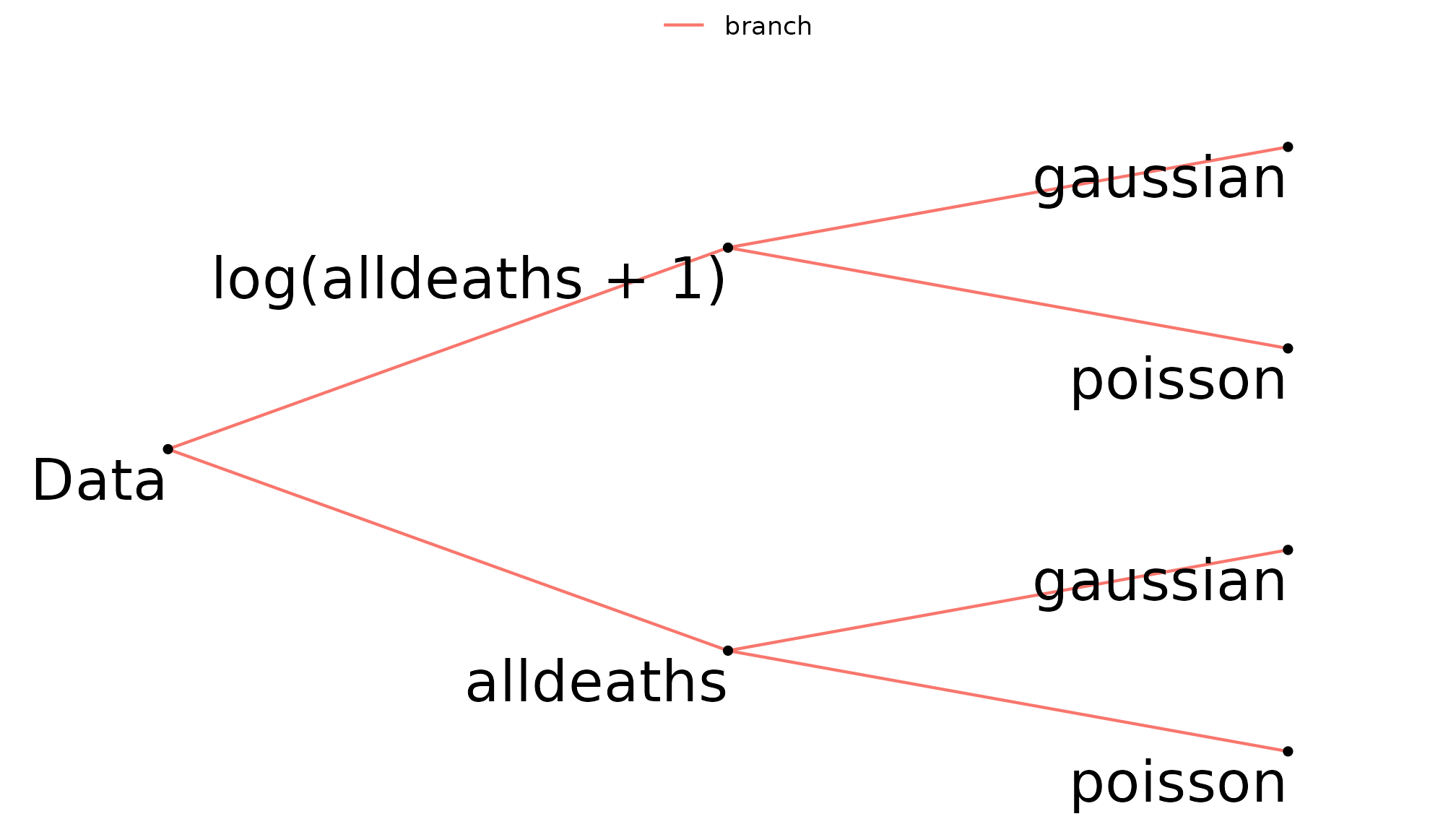
In order to specify that hurricane_mv should only
contain analyses where log(alldeaths + 1) is modelled using
a Gaussian and alldeaths modelled using Poisson we can use
branch_condition() and add_branch_condition()
to add it to hurricane_mv.
match_poisson <- branch_condition(alldeaths, poisson)

match_log_lin <- branch_condition(log(alldeaths + 1), gaussian)

hurricane_mv <- add_branch_condition(hurricane_mv, match_poisson, match_log_lin)
The multiverse tree shows that log(alldeaths + 1) will
only be modelled as Gaussian and alldeaths will
only be modelled as Poisson.
multiverse_tree(hurricane_mv, label = "code", c("dep_var", "distributions"))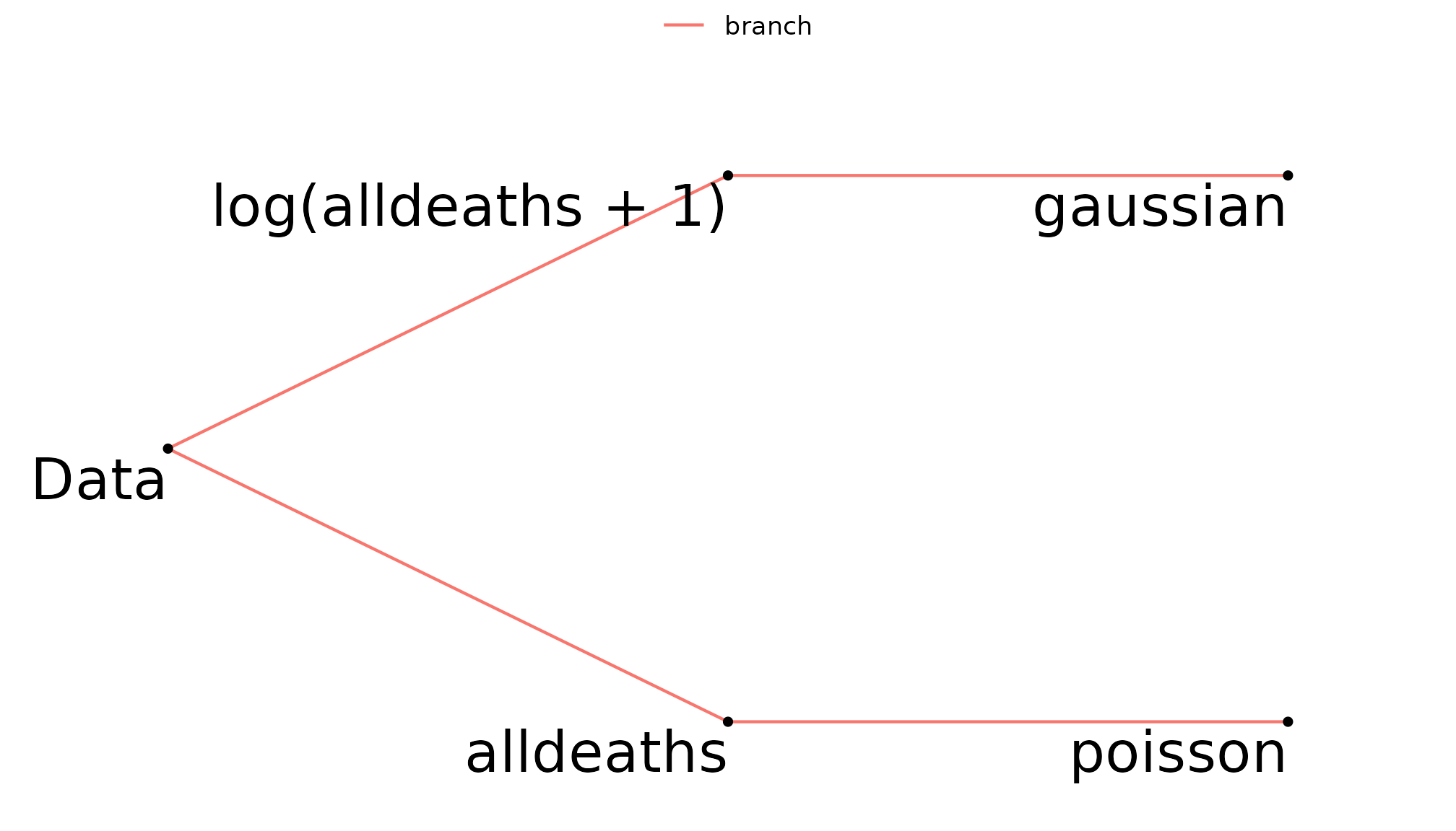
glm_mverse(hurricane_mv)

summary(hurricane_mv)
## # A tibble: 24 × 18
##    universe femininity_branch damage_branch models_branch distributions_branch
##    <fct>    <fct>             <fct>         <fct>         <fct>
##  1 1        binary_gender     damage_orig   models_1      distributions_1
##  2 1        binary_gender     damage_orig   models_1      distributions_1
##  3 1        binary_gender     damage_orig   models_1      distributions_1
##  4 2        binary_gender     damage_orig   models_1      distributions_2
##  5 2        binary_gender     damage_orig   models_1      distributions_2
##  6 2        binary_gender     damage_orig   models_1      distributions_2
##  7 3        binary_gender     damage_log    models_1      distributions_1
##  8 3        binary_gender     damage_log    models_1      distributions_1
##  9 3        binary_gender     damage_log    models_1      distributions_1
## 10 4        binary_gender     damage_log    models_1      distributions_2
## # ℹ 14 more rows
## # ℹ 13 more variables: dep_var_branch <fct>, term <chr>, estimate <dbl>,
## #   std.error <dbl>, statistic <dbl>, p.value <dbl>, conf.low <dbl>,
## #   conf.high <dbl>, femininity_branch_code <fct>, damage_branch_code <fct>,
## #   models_branch_code <fct>, distributions_branch_code <fct>,
## #   dep_var_branch_code <fct>
A summary of the 24 models on the femininity
coefficients is shown in the specification curve.
spec_summary(hurricane_mv, var = "femininity") |>
  spec_curve(label = "code", spec_matrix_spacing = 4) +
  labs(colour = "Significant at 0.05") +
  theme(legend.position = "top")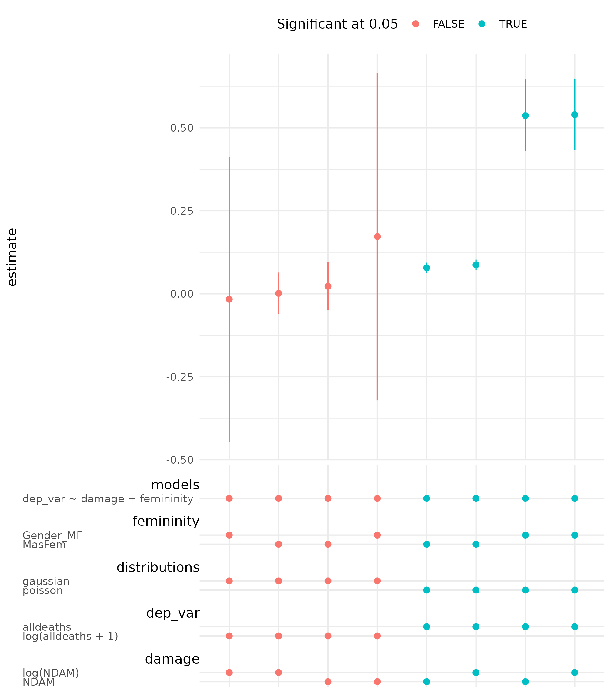
Negative Binomial Regression
Jung et al. (2014) used negative
binomial regression to analyse the severity of female versus male
hurricane names on number of deaths. In this section we will
glm.nb_mverse() to do a similar analysis.
First, let’s setup the multiverse of analyses.
hurricane_nb_mv <- create_multiverse(hurricane)

femininity <- mutate_branch(binary_gender = Gender_MF,
                            cts_gender = MasFem)

damage <- mutate_branch(damage_orig = NDAM,
                        damage_log = log(NDAM))

models <- formula_branch(alldeaths ~ damage + femininity)

hurricane_nb_mv <- hurricane_nb_mv |>
  add_mutate_branch(femininity, damage) |>
  add_formula_branch(models)
A summary of hurricane_nb_mv shows the four models in
the multiverse.
summary(hurricane_nb_mv)
## # A tibble: 4 × 7
##   universe femininity_branch damage_branch models_branch femininity_branch_code
##   <fct>    <fct>             <fct>         <fct>         <fct>
## 1 1        binary_gender     damage_orig   models_1      Gender_MF
## 2 2        binary_gender     damage_log    models_1      Gender_MF
## 3 3        cts_gender        damage_orig   models_1      MasFem
## 4 4        cts_gender        damage_log    models_1      MasFem
## # ℹ 2 more variables: damage_branch_code <fct>, models_branch_code <fct>
Next, use glm.nb_mverse() to fit the negative binomial
regressions.
glm.nb_mverse(hurricane_nb_mv)
summary(hurricane_nb_mv)
## # A tibble: 12 × 14
## universe femininity_branch damage_branch models_branch term estimate
## <fct> <fct> <fct> <fct> <chr> <dbl>
## 1 1 binary_gender damage_orig models_1 (Intercept) 1.71
## 2 1 binary_gender damage_orig models_1 damage 0.0000981
## 3 1 binary_gender damage_orig models_1 femininity 0.227
## 4 2 binary_gender damage_log models_1 (Intercept) -1.96
## 5 2 binary_gender damage_log models_1 damage 0.577
## 6 2 binary_gender damage_log models_1 femininity 0.108
## 7 3 cts_gender damage_orig models_1 (Intercept) 1.66
## 8 3 cts_gender damage_orig models_1 damage 0.0000983
## 9 3 cts_gender damage_orig models_1 femininity 0.0304
## 10 4 cts_gender damage_log models_1 (Intercept) -2.05
## 11 4 cts_gender damage_log models_1 damage 0.576
## 12 4 cts_gender damage_log models_1 femininity 0.0240
## # ℹ 8 more variables: std.error <dbl>, statistic <dbl>, p.value <dbl>,
## # conf.low <dbl>, conf.high <dbl>, femininity_branch_code <fct>,
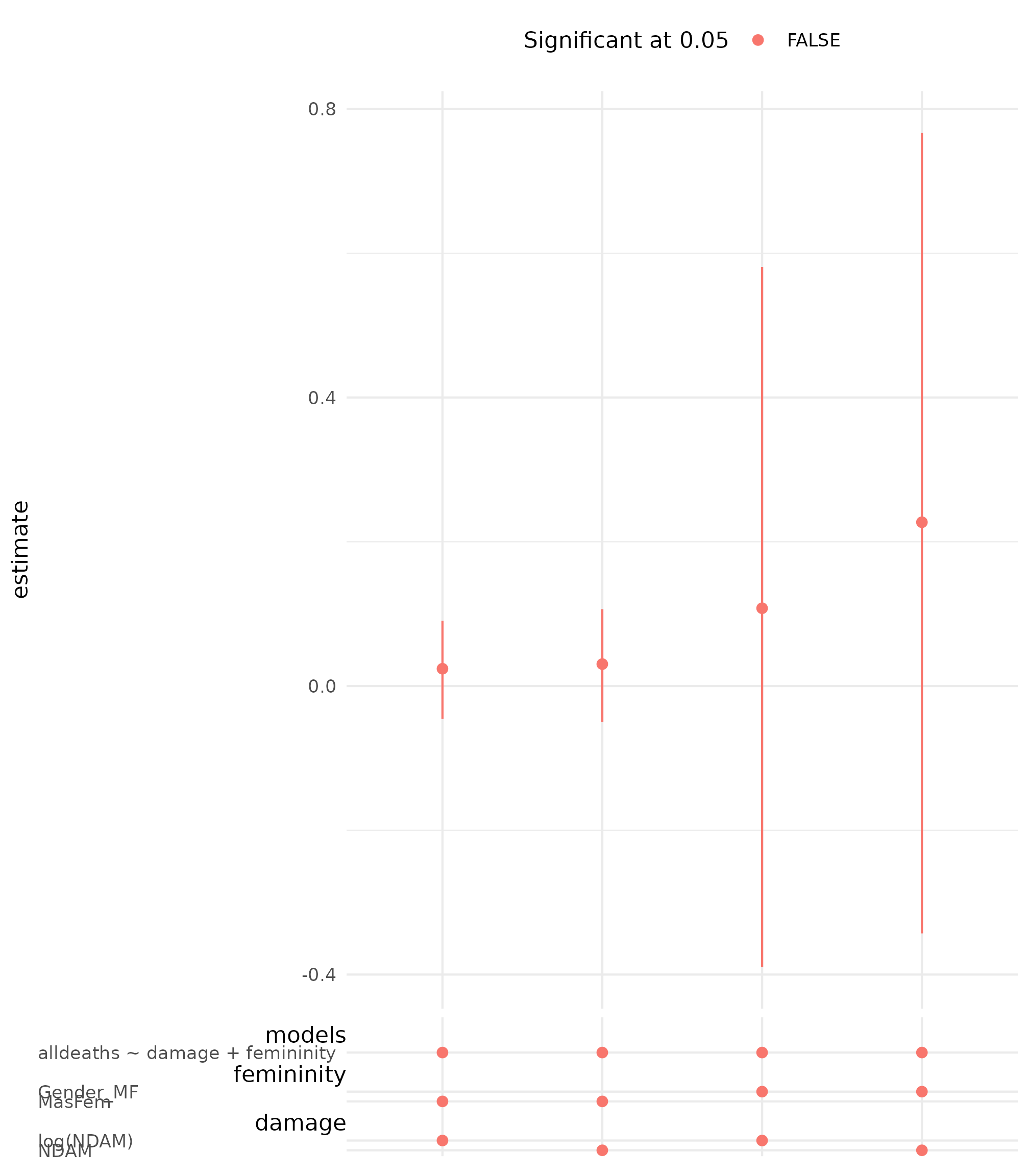
## # damage_branch_code <fct>, models_branch_code <fct>Finally, we can plot the specification curve.
spec_summary(hurricane_nb_mv, var = "femininity") |>
  spec_curve(label = "code", spec_matrix_spacing = 4) +
  labs(colour = "Significant at 0.05") +
  theme(legend.position = "top")