Basic Regressions with mverse
Source:vignettes/mverse_intro_regressionmodelling.Rmd
mverse_intro_regressionmodelling.RmdThis vignette describes the workflow of linear regression modeling in the multiverse with the following functions:
-
formula_branch(),add_formula_branch: create branches for regression formulas and add them to amverseobject. -
lm_mverse(): fit a simple linear model with the given formula branches and family branches. -
summary(): provide a summary of the fitted models in different branches. -
spec_curve(): display the specification curve of a model.
We will use the Boston housing dataset {Harrison Jr and Rubinfeld (1978)} as an example.
This dataset has 506 observations on 14 variables. This dataset is
extensively used in regression analyses and algorithm benchmarks. The
objective is to predict the median value of a home (medv)
with the feature variables.
dplyr::glimpse(MASS::Boston) # using kable for displaying data in html
## Rows: 506
## Columns: 14
## $ crim    <dbl> 0.00632, 0.02731, 0.02729, 0.03237, 0.06905, 0.02985, 0.08829,…
## $ zn      <dbl> 18.0, 0.0, 0.0, 0.0, 0.0, 0.0, 12.5, 12.5, 12.5, 12.5, 12.5, 1…
## $ indus   <dbl> 2.31, 7.07, 7.07, 2.18, 2.18, 2.18, 7.87, 7.87, 7.87, 7.87, 7.…
## $ chas    <int> 0, 0, 0, 0, 0, 0, 0, 0, 0, 0, 0, 0, 0, 0, 0, 0, 0, 0, 0, 0, 0,…
## $ nox     <dbl> 0.538, 0.469, 0.469, 0.458, 0.458, 0.458, 0.524, 0.524, 0.524,…
## $ rm      <dbl> 6.575, 6.421, 7.185, 6.998, 7.147, 6.430, 6.012, 6.172, 5.631,…
## $ age     <dbl> 65.2, 78.9, 61.1, 45.8, 54.2, 58.7, 66.6, 96.1, 100.0, 85.9, 9…
## $ dis     <dbl> 4.0900, 4.9671, 4.9671, 6.0622, 6.0622, 6.0622, 5.5605, 5.9505…
## $ rad     <int> 1, 2, 2, 3, 3, 3, 5, 5, 5, 5, 5, 5, 5, 4, 4, 4, 4, 4, 4, 4, 4,…
## $ tax     <dbl> 296, 242, 242, 222, 222, 222, 311, 311, 311, 311, 311, 311, 31…
## $ ptratio <dbl> 15.3, 17.8, 17.8, 18.7, 18.7, 18.7, 15.2, 15.2, 15.2, 15.2, 15…
## $ black   <dbl> 396.90, 396.90, 392.83, 394.63, 396.90, 394.12, 395.60, 396.90…
## $ lstat   <dbl> 4.98, 9.14, 4.03, 2.94, 5.33, 5.21, 12.43, 19.15, 29.93, 17.10…
## $ medv    <dbl> 24.0, 21.6, 34.7, 33.4, 36.2, 28.7, 22.9, 27.1, 16.5, 18.9, 15…
Simple Linear Regression with mverse
In order to perform a linear regression in the multiverse, we create
a formula branch with all the models we wish to explore, add it the
mverse object, and execute lm on each universe
by calling lm_mverse.
Create a multiverse with mverse.
mv <- create_multiverse(MASS::Boston)We can explore models of the median value of home prices
medv on different combinations of the following explanatory
variables: proportion of adults without some high school education and
proportion of male workers classified as laborers (lstat),
average number of rooms per dwelling (rm), per capita crime
rate (crim), and property tax (tax).
Create the models with formula_branch()
formulas <- formula_branch(medv ~ log(lstat) * rm,
                           medv ~ log(lstat) * tax,
                           medv ~ log(lstat) * tax * rm)
Add the models to the multiverse mv.
mv <- mv |> add_formula_branch(formulas)Fit lm() across mv using
lm_mverse().
lm_mverse(mv)By default, summary will give the estimates of
parameters for each model. You can also output other information by
changing the output parameter.
summary(mv)
## # A tibble: 16 × 10
##    universe formulas_branch term  estimate std.error statistic  p.value conf.low
##    <fct>    <fct>           <chr>    <dbl>     <dbl>     <dbl>    <dbl>    <dbl>
##  1 1        formulas_1      (Int… -2.49e+1   6.66        -3.74 2.07e- 4 -3.80e+1
##  2 1        formulas_1      log(…  1.16e+1   2.61         4.45 1.05e- 5  6.50e+0
##  3 1        formulas_1      rm     1.10e+1   0.973       11.3  2.08e-26  9.05e+0
##  4 1        formulas_1      log(… -3.35e+0   0.405       -8.29 1.04e-15 -4.15e+0
##  5 2        formulas_2      (Int…  4.62e+1   2.83        16.3  1.89e-48  4.07e+1
##  6 2        formulas_2      log(… -9.60e+0   1.15        -8.31 9.04e-16 -1.19e+1
##  7 2        formulas_2      tax    1.35e-2   0.00750      1.80 7.23e- 2 -1.23e-3
##  8 2        formulas_2      log(… -6.35e-3   0.00278     -2.28 2.29e- 2 -1.18e-2
##  9 3        formulas_3      (Int… -1.88e+2  15.4        -12.2  3.36e-30 -2.18e+2
## 10 3        formulas_3      log(…  5.23e+1   6.70         7.80 3.73e-14  3.91e+1
## 11 3        formulas_3      tax    3.82e-1   0.0344      11.1  7.46e-26  3.15e-1
## 12 3        formulas_3      rm     3.10e+1   2.30        13.5  1.98e-35  2.65e+1
## 13 3        formulas_3      log(… -1.00e-1   0.0135      -7.40 5.89e-13 -1.27e-1
## 14 3        formulas_3      log(… -7.30e+0   1.06        -6.86 2.04e-11 -9.40e+0
## 15 3        formulas_3      tax:… -4.84e-2   0.00529     -9.16 1.32e-18 -5.88e-2
## 16 3        formulas_3      log(…  1.07e-2   0.00216      4.96 9.62e- 7  6.49e-3
## # ℹ 2 more variables: conf.high <dbl>, formulas_branch_code <fct>
Changing output to df yields the degrees of
freedom table.
summary(mv, output = "df")
##   universe formulas_branch p n.minus.p p.star         formulas_branch_code
## 1        1      formulas_1 4       502      4       medv ~ log(lstat) * rm
## 2        2      formulas_2 4       502      4      medv ~ log(lstat) * tax
## 3        3      formulas_3 8       498      8 medv ~ log(lstat) * tax * rm
Other options include F (output = "f") statistics
summary(mv, output = "f")
##   universe formulas_branch    value numdf dendf         formulas_branch_code
## 1        1      formulas_1 482.2512     3   502       medv ~ log(lstat) * rm
## 2        2      formulas_2 341.0488     3   502      medv ~ log(lstat) * tax
## 3        3      formulas_3 367.7342     7   498 medv ~ log(lstat) * tax * rm
and
(output = "r").
# output R-squared by `r.squared` or "r"
summary(mv, output = "r")
## universe formulas_branch r.squared adj.r.squared formulas_branch_code
## 1 1 formulas_1 0.7423994 0.7408600 medv ~ log(lstat) * rm
## 2 2 formulas_2 0.6708513 0.6688842 medv ~ log(lstat) * tax
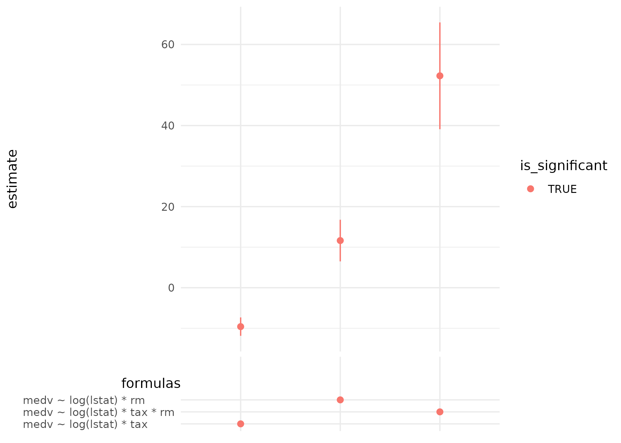
## 3 3 formulas_3 0.8378980 0.8356194 medv ~ log(lstat) * tax * rmFinally, we can display how the effect of number of rooms in a
dwelling log(lstat) using spec_curve.
spec_summary(mv, var = "log(lstat)") |>
  spec_curve(label = "code") +
  ggplot2::labs("Significant at 0.05")